R for reproducible scientific analysis

Dataframe manipulation with dplyr

Manipulation of dataframes means many things to many researchers, we often select certain observations (rows) or variables (columns), we often group the data by a certain variable(s), or we even calculate summary statistics. We can do these operations using the normal base R operations:

mean(gapminder[gapminder$continent == "Africa", "gdpPercap"])

[1] 2193.755

mean(gapminder[gapminder$continent == "Americas", "gdpPercap"])

[1] 7136.11

mean(gapminder[gapminder$continent == "Asia", "gdpPercap"])

[1] 7902.15

But this isn’t very nice because there is a fair bit of repetition. Repeating yourself will cost you time, both now and later, and potentially introduce some nasty bugs.

The dplyr package

Luckily, the dplyr package provides a number of very useful functions for manipulating dataframes in a way that will reduce the above repetition, reduce the probability of making errors, and probably even save you some typing. As an added bonus, you might even find the dplyr grammar easier to read.

Here we’re going to cover 6 of the most commonly used functions as well as using pipes (%>%) to combine them.

1. select()
2. filter()
3. group_by()
4. summarize()
5. mutate()

If you have have not installed this package earlier, please do so:

install.packages('dplyr')

Now let’s load the package:

library(dplyr)

Using select()

If, for example, we wanted to move forward with only a few of the variables in our dataframe we could use the select() function. This will keep only the variables you select.

year_country_gdp <- select(gapminder,year,country,gdpPercap)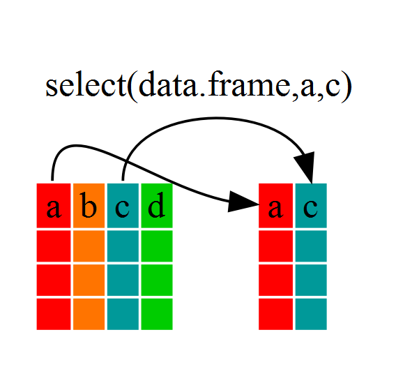

If we open up year_country_gdp we’ll see that it only contains the year, country and gdpPercap. Above we used ‘normal’ grammar, but the strengths of dplyr lie in combining several functions using pipes. Since the pipes grammar is unlike anything we’ve seen in R before, let’s repeat what we’ve done above using pipes.

year_country_gdp <- gapminder %>% select(year,country,gdpPercap)

To help you understand why we wrote that in that way, let’s walk through it step by step. First we summon the gapminder dataframe and pass it on, using the pipe symbol %>%, to the next step, which is the select() function. In this case we don’t specify which data object we use in the select() function since in gets that from the previous pipe. Fun Fact: There is a good chance you have encountered pipes before in the shell. In R, a pipe symbol is %>% while in the shell it is | but the concept is the same!

Using filter()

If we now wanted to move forward with the above, but only with European countries, we can combine select and filter

europe <- gapminder %>%
    filter(continent == "Europe") %>%
    select(year,country,gdpPercap)
# Check that we've only got data for European countries
unique(europe$country)

 [1] Albania                Austria                Belgium               
 [4] Bosnia and Herzegovina Bulgaria               Croatia               
 [7] Czech Republic         Denmark                Finland               
[10] France                 Germany                Greece                
[13] Hungary                Iceland                Ireland               
[16] Italy                  Montenegro             Netherlands           
[19] Norway                 Poland                 Portugal              
[22] Romania                Serbia                 Slovak Republic       
[25] Slovenia               Spain                  Sweden                
[28] Switzerland            Turkey                 United Kingdom        
142 Levels: Afghanistan Albania Algeria Angola Argentina ... Zimbabwe

Note that its possible to filter by multiple criteria with a single instance of filter(). For instance, if we wanted to remove the UK from Europe, it’s as simple as adding an extra criteria to filter with & (no referendum required!). If we wanted to get entries where either condition was true, we would use |.

europe <- gapminder %>%
    filter(continent == "Europe" & country != "United Kingdom") %>%
    select(year,country,gdpPercap)
unique(europe$country)

 [1] Albania                Austria                Belgium               
 [4] Bosnia and Herzegovina Bulgaria               Croatia               
 [7] Czech Republic         Denmark                Finland               
[10] France                 Germany                Greece                
[13] Hungary                Iceland                Ireland               
[16] Italy                  Montenegro             Netherlands           
[19] Norway                 Poland                 Portugal              
[22] Romania                Serbia                 Slovak Republic       
[25] Slovenia               Spain                  Sweden                
[28] Switzerland            Turkey                
142 Levels: Afghanistan Albania Algeria Angola Argentina ... Zimbabwe

As with last time, first we pass the gapminder dataframe to the filter() function, then we pass the filtered version of the gapminder dataframe to the select() function. Note: The order of operations is very important in this case. If we used ‘select’ first, filter would not be able to find the variable continent since we would have removed it in the previous step.

Using group_by() and summarize()

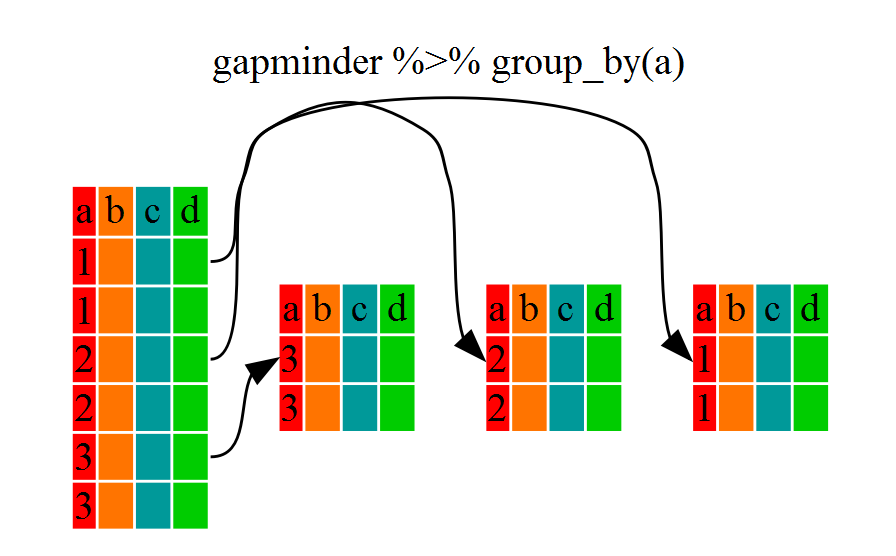
Now, we were supposed to be reducing the error prone repetitiveness of what can be done with base R, but up to now we haven’t done that since we would have to repeat the above for each continent. Instead of filter(), which will only pass observations that meet your criteria (in the above: continent=="Europe"), we can use group_by(), which will essentially use every unique criteria that you could have used in filter.

str(gapminder)

'data.frame':   1704 obs. of  6 variables:
 $ country  : Factor w/ 142 levels "Afghanistan",..: 1 1 1 1 1 1 1 1 1 1 ...
 $ year     : int  1952 1957 1962 1967 1972 1977 1982 1987 1992 1997 ...
 $ pop      : num  8425333 9240934 10267083 11537966 13079460 ...
 $ continent: Factor w/ 5 levels "Africa","Americas",..: 3 3 3 3 3 3 3 3 3 3 ...
 $ lifeExp  : num  28.8 30.3 32 34 36.1 ...
 $ gdpPercap: num  779 821 853 836 740 ...

str(gapminder %>% group_by(continent))

Classes 'grouped_df', 'tbl_df', 'tbl' and 'data.frame': 1704 obs. of  6 variables:
 $ country  : Factor w/ 142 levels "Afghanistan",..: 1 1 1 1 1 1 1 1 1 1 ...
 $ year     : int  1952 1957 1962 1967 1972 1977 1982 1987 1992 1997 ...
 $ pop      : num  8425333 9240934 10267083 11537966 13079460 ...
 $ continent: Factor w/ 5 levels "Africa","Americas",..: 3 3 3 3 3 3 3 3 3 3 ...
 $ lifeExp  : num  28.8 30.3 32 34 36.1 ...
 $ gdpPercap: num  779 821 853 836 740 ...
 - attr(*, "vars")=List of 1
  ..$ : symbol continent
 - attr(*, "drop")= logi TRUE
 - attr(*, "indices")=List of 5
  ..$ : int  24 25 26 27 28 29 30 31 32 33 ...
  ..$ : int  48 49 50 51 52 53 54 55 56 57 ...
  ..$ : int  0 1 2 3 4 5 6 7 8 9 ...
  ..$ : int  12 13 14 15 16 17 18 19 20 21 ...
  ..$ : int  60 61 62 63 64 65 66 67 68 69 ...
 - attr(*, "group_sizes")= int  624 300 396 360 24
 - attr(*, "biggest_group_size")= int 624
 - attr(*, "labels")='data.frame':  5 obs. of  1 variable:
  ..$ continent: Factor w/ 5 levels "Africa","Americas",..: 1 2 3 4 5
  ..- attr(*, "vars")=List of 1
  .. ..$ : symbol continent
  ..- attr(*, "drop")= logi TRUE

You will notice that the structure of the dataframe where we used group_by() (grouped_df) is not the same as the original gapminder (data.frame). A grouped_df can be thought of as a list where each item in the listis a data.frame which contains only the rows that correspond to the a particular value continent (at least in the example above).

Using summarize()

The above was a bit on the uneventful side because group_by() much more exciting in conjunction with summarize(). This will allow use to create new variable(s) by using functions that repeat for each of the continent-specific data frames. That is to say, using the group_by() function, we split our original dataframe into multiple pieces, then we can run functions (e.g. mean() or sd()) within summarize().

gdp_bycontinents <- gapminder %>%
    group_by(continent) %>%
    summarize(mean_gdpPercap=mean(gdpPercap))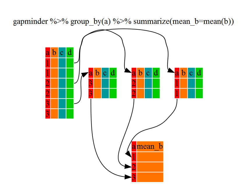

That allowed us to calculate the mean gdpPercap for each continent, but it gets even better.

The function group_by() allows us to group by multiple variables. Let’s group by year and continent.

gdp_bycontinents_byyear <- gapminder %>%
    group_by(continent,year) %>%
    summarize(mean_gdpPercap=mean(gdpPercap))

That is already quite powerful, but it gets even better! You’re not limited to defining 1 new variable in summarize().

gdp_pop_bycontinents_byyear <- gapminder %>%
    group_by(continent,year) %>%
    summarize(mean_gdpPercap=mean(gdpPercap),
              sd_gdpPercap=sd(gdpPercap),
              mean_pop=mean(pop),
              sd_pop=sd(pop))

Using mutate()

We can also create new variables prior to (or even after) summarizing information using mutate().

gdp_pop_bycontinents_byyear <- gapminder %>%
    mutate(gdp_billion=gdpPercap*pop/10^9) %>%
    group_by(continent,year) %>%
    summarize(mean_gdpPercap=mean(gdpPercap),
              sd_gdpPercap=sd(gdpPercap),
              mean_pop=mean(pop),
              sd_pop=sd(pop),
              mean_gdp_billion=mean(gdp_billion),
              sd_gdp_billion=sd(gdp_billion))

year_country_lifeExp_Africa <- gapminder %>%
                           filter(continent=="Africa") %>%
                           select(year,country,lifeExp)

lifeExp_bycountry <- gapminder %>%
   group_by(country) %>%
   summarize(mean_lifeExp=mean(lifeExp))

lifeExp_2countries_bycontinents <- gapminder %>% 
   filter(year==2002) %>%
   group_by(continent) %>%
   sample_n(2) %>%
   summarize(mean_lifeExp=mean(lifeExp)) %>%
   arrange(desc(mean_lifeExp))

Other great resources

Data Wrangling Cheat sheet Introduction to dplyr