
R for reproducible scientific analysis
Project management with RStudio
Learning Objectives
- To be able to create self-contained projects in RStudio
- To be able to use git from within RStudio
Introduction
The scientific process is naturally incremental, and many projects start life as random notes, some code, then a manuscript, and eventually everything is a bit mixed together.
Managing your projects in a reproducible fashion doesn’t just make your science reproducible, it makes your life easier.
— Vince Buffalo (@vsbuffalo) April 15, 2013
Most people tend to organize their projects like this:
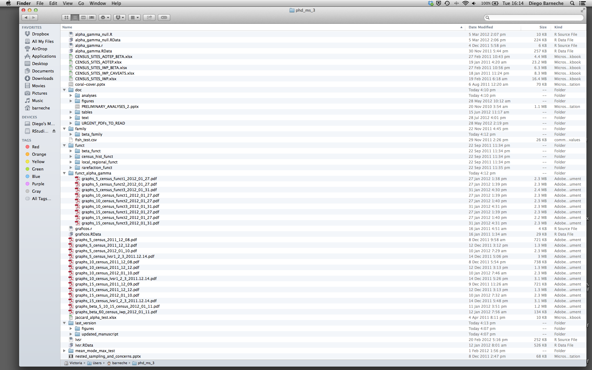
There are many reasons why we should ALWAYS avoid this:
- It is really hard to tell which version of your data is the original and which is the modified;
- It gets really messy because it mixes files with various extensions together;
- It probably takes you a lot of time to actually find things, and relate the correct figures to the exact code that has been used to generate it;
A good project layout will ultimately make your life easier:
- It will help ensure the integrity of your data;
- It makes it simpler to share your code with someone else (a lab-mate, collaborator, or supervisor);
- It allows you to easily upload your code with your manuscript submission;
- It makes it easier to pick the project back up after a break.
A possible solution
Fortunately, there are tools and packages which can help you manage your work effectively.
One of the most powerful and useful aspects of RStudio is its project management functionality. We’ll be using this today to create a self-contained, reproducible project.
Challenge: Creating a self-contained project
We’re going to create a new project in RStudio:
- Click the “File” menu button, then “New Project”.
- Click “New Directory”.
- Click “Empty Project”.
- Type in the name of the directory to store your project, e.g. “my_project”.
- Make sure that the checkbox for “Create a git repository” is selected.
- Click the “Create Project” button.
Now when we start R in this project directory, or open this project with RStudio, all of our work on this project will be entirely self-contained in this directory.
Best practices for project organisation
Although there is no “best” way to lay out a project, there are some general principles to adhere to that will make project management easier:
Treat data as read only
This is probably the most important goal of setting up a project. Data is typically time consuming and/or expensive to collect. Working with them interactively (e.g., in Excel) where they can be modified means you are never sure of where the data came from, or how it has been modified since collection. It is therefore a good idea to treat your data as “read-only”.
Data Cleaning
In many cases your data will be “dirty”: it will need significant preprocessing to get into a format R (or any other programming language) will find useful. This task is sometimes called “data munging”. I find it useful to store these scripts in a separate folder, and create a second “read-only” data folder to hold the “cleaned” data sets.
Treat generated output as disposable
Anything generated by your scripts should be treated as disposable: it should all be able to be regenerated from your scripts.
There are lots of different ways to manage this output. I find it useful to have an output folder with different sub-directories for each separate analysis. This makes it easier later, as many of my analyses are exploratory and don’t end up being used in the final project, and some of the analyses get shared between projects.
Separate function definition and application
The most effective way I find to work in R, is to play around in the interactive session, then copy commands across to a script file when I’m sure they work and do what I want. You can also save all the commands you’ve entered using the history command, but I don’t find it useful because when I’m typing its 90% trial and error.
When your project is new and shiny, the script file usually contains many lines of directly executed code. As it matures, reusable chunks get pulled into their own functions. It’s a good idea to separate these into separate folders; one to store useful functions that you’ll reuse across analyses and projects, and one to store the analysis scripts.
Save the data in the data directory
Now we have a good directory structure we will now place/save the data file in the data/ directory.
Challenge 1
Download the gapminder data from here.
- Download the file (CTRL + S, right mouse click -> “Save as”, or File -> “Save page as”)
- Make sure it’s saved under the name
gapminder-FiveYearData.csv - Save the file in the
data/folder within your project.
We will load and inspect these data later.
Challenge 2
It is useful to get some general idea about the dataset, directly from the command line, before loading it into R. Understanding the dataset better will come handy when making decisions on how to load it in R. Use command-line shell to answer the following questions: 1. What is the size of the file? 2. How many rows of data does it contain? 3. What are the data types of values stored in this file?
Version Control
We also set up our project to integrate with git, putting it under version control. RStudio has a nicer interface to git than shell, but is very limited in what it can do, so you will find yourself occasionally needing to use the shell. Let’s go through and make an initial commit of our template files.
The workspace/history pane has a tab for “Git”. We can stage each file by checking the box: you will see a Green “A” next to stage files and folders, and yellow question marks next to files or folders git doesn’t know about yet. RStudio also nicely shows you the difference between files from different commits.
Challenge 3
- Create a directory within your project called
graphs. - Modify the
.gitignorefile to containgraphs/so that this disposable output isn’t versioned.
Add the newly created folders to version control using the git interface.